Customer Segmentation using Machine Learning
In this blog post, I will create a customer segmentation report by applying various unsupervised and supervised machine learning methods. This project is the final assignment of Udacity’s Data Science Nanodegree.
I Introduction
Identifying different customer segments is a common problem in the domain of marketing. This classification can often be made based on various demographic data. Using a German mail-order sales company’s data set, I will first create clusters based on demographic data of the total population. I will then compare these with the customer data to determine which groups of people are particularly frequent customers for this company.
The second part of the project is to predict whether customers will respond to particular marketing activity and become customers or not. The conclusion of this part is the participation in a Kaggle competition, where my model will compete with others.
First, I will go into the dataset and perform several cleaning steps (II). This is followed by the Customer Segmentation Report (III) and the Supervised Learning Part (IV). Finally, I will briefly summarize my findings. The complete code for this project can be found in my GitHub repository, which I link at the end. Now have fun reading!
II Data Understanding and Cleaning
The demographic data set consisted of 891,221 observations and 366 columns. The customer dataset originally consisted of 191,652 observations and 369 columns. The three additional columns were “PRODUCT_GROUP”, “CUSTOMER_GROUP”, “ONLINE_PURCHASE”. To get an overview of the dataset, I created a DataFrame that contains the following meta-information:
- na_percentage: The percentage of NaN values per column
- dtypes: Data types of the column
- n_dtypes: Unique data types per column
- unique_values: Unique values per column
- description: Column descriptions from the additional Excel files
Six of the columns had two data types instead of one, which had to be considered during the cleaning process. The majority of columns had a NaN percentage of 0.2 or less (see Figure 1). The highest NaN values (more than 0.9) were in the columns containing information about the age of the children.

The following columns were created by manually working through the additional Excel files. These included the features, their descriptions, and values that the features could assume.
- type: Feature type (Numerical, Ordinal, Categorical, Binary or Unknown)
- 9 unknown: If “unknown” value is coded as 9
- 0 unknown: If “unknown” value is coded as 0
- -1 unknown: If “unknown” value is coded as -1
- action: Preprocessing action
- reason: Reason for action
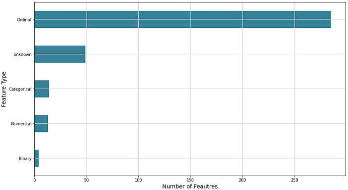
I found out that most of the columns were ordinal, which means ordered categorical features (see Figure 2).
Based on the meta table a preprocessing function was defined. The respective steps can be seen in Figure 3.

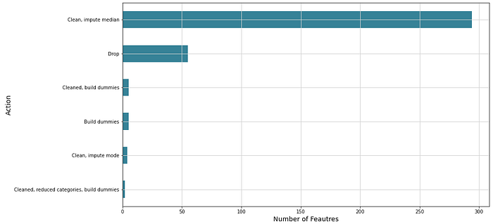
Since most of the values were ordinal, the most common cleaning process was “Clean, impute median” (see Figure 4). 49 columns were dropped because they had no description, 5 because they exceeded the nan threshold, and one column CAMEO_DEU_2015 because it had too many categories. There were six columns that contained more than one data type and therefore needed special attention during the cleaning process (for more detail check the excel file in my GitHub repo). These columns all contained either date information or textual labels for the categories (str datatype). The NaN entries had the float data type.
5 columns were used to create dummies. This led to a final column number of 372. Also, 139,890 rows were dropped because they had more than 10 percent nan values, which resulted in 751,331 rows.
Before approaching clustering, I applied standard scaling since it was essential for many machine learning algorithms, especially for Principal Component Analysis (PCA). There are several scaling methods on sklearn, like RobustScaler, Normalizer or MinMaxScaler. For PCA, data should be transformed so that zero mean and unit variance should be guaranteed. In this case, the StandardScaler is the most suitable.
III Customer Segmentation Report
To define different demographic clusters and find out which of them are particularly strongly represented in the customer dataset, I use a k-means clustering method. Before that, I will use PCA to reduce both datasets’ feature dimensions. Finally, I will briefly interpret my results.
1. Principal Component Analysis
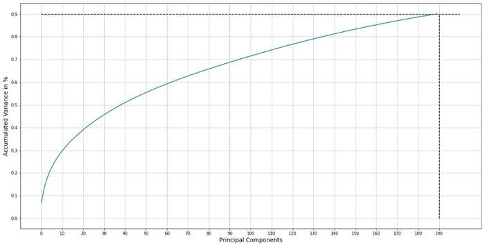
Before actually clustering the data, I applied PCA to reduce the dimensionality. In this multivariate statistic method, a large number of statistical variables are approximated by a smaller number of linear combinations that are as meaningful as possible. I selected a value of 0.9 for the explained variance. This means that the number of principal components are chosen to explain 90 percent of the variance in the data set. The analysis showed that this reduced the number of dimensions from 372 to 190 (see Figure 5).
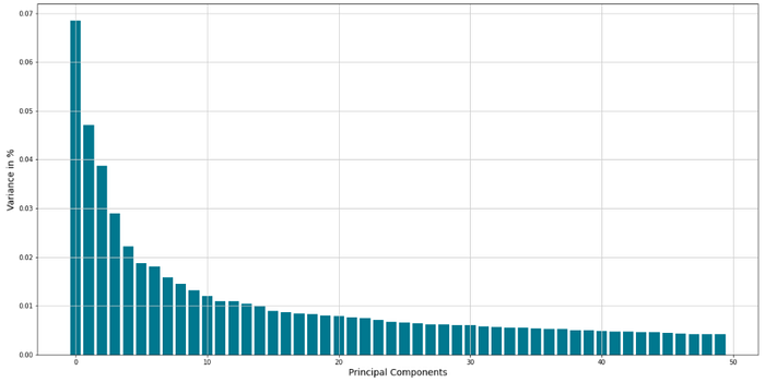
The principal components are shown sorted by explained variance. Figure 6 shows that especially the first four principal components explain relatively much variance.
It is possible to analyze the influence of the original features on the individual principal components, which I will do in the first component (PC1) to demonstrate the concept.
High positive influence on PC1:
- MOBI_REGIO: This feature represents the moving patterns of a person. The lower the value, the higher the mobility.
- LP_LEBENSPHASE_GROB: This feature represents the phase of a person’s life. The higher the value, the higher the income and the higher the age of a person.
- KBA05_ANHANG: This feature indicates how many trailers are present in a microcell. The higher the value, the more trailers are present.
High negative influence on PC1:
- HH_EINKOMMEN_SCORE: This is the estimated household net income. The higher the value the lower the income.
- PLZ8_ANTG1: The number of 1–2 family houses in the zip code area.
- OST_WEST_KZ: This indicates whether a person is from the former GDR (German Democratic Republic) or from the FRG (Federal Republic of Germany).
In summary, PC1 one is positively influenced when individuals are less mobile, old, and have a high income.
2. K-Means Clustering
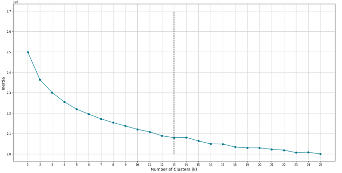
Using the 190 principal components, I used a k-means approach to perform clustering on the data. First, I wanted to find the optimal number of clusters k. I tested a range of 1 to 25 clusters, each time saving the inertia, which is the sum of samples’ squared distances to their closest cluster center. I then plotted the inertias for each k (see Figure 7). The elbow method is a good, if not entirely accurate, way to determine the optimal number of clusters. The elbow point is when adding more clusters only leads to diminishing returns, i.e., where the curve begins to flatten. I have set the elbow point to 13, which indicates that the optimal number of clusters k is 13.
To determine which demographic clusters are particularly prevalent in the customer dataset, I first formed 13 clusters from the demographic dataset. I then cleaned, scaled, and PCA-transformed the customer data. I then used the k-means model to assign one of 13 labels to each data point in the customer dataset. A comparison of the proportion per cluster and data set can be seen in Figure 8.

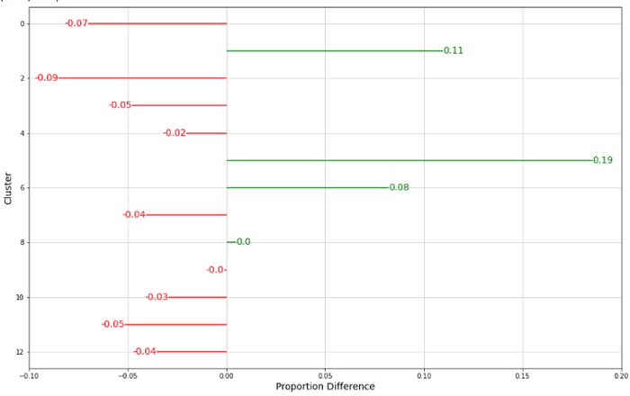
It can be seen that especially 3 clusters are dominant. Figure 9 shows the difference of proportion in the customer dataset and the demographic dataset. This graph also confirms that 3 clusters are particularly strongly represented. These are clusters 1, 5, and 6.
3. Cluster Interpretation
To analyze the clusters, I grouped the labeled customer dataset by cluster and calculated each feature’s mean. Then I iterated through the features and created a DataFrame containing the clusters with the three highest and the three lowest mean values for each feature. Then, for the clusters representing the dominant customer segments, I analyzed for which features they were the cluster with the highest and lowest average scores, respectively. In the following, I would like to show what my results imply for clusters 1, 5 and 6. I will describe the customer segments. The features in detail can be seen on GitHub.
Cluster 1
This cluster represents the upper middle class with a high income. Members of this customer segment tend to be less mobile, have a relatively large number of children, and are predominantly fixated on their own homes. People from this cluster live in areas with low unemployment. The formative youth years of this group were primarily the 1970s.
Cluster 5
This cluster has the highest proportion of academics and top earners. Compared to cluster 1, members appear to be older because their formative teenage years were the 1950s, where they often belonged to the “green avant-garde.” Members of this group live in very good neighborhoods. People from this category are not very dreamy and are characterized by high financial interest, which translates into a high probability of being an investor.
Cluster 6
Cluster 6 is more urban, with more German-sounding names, and tends to be from western Germany. They are often golden agers, i.e., people over 50 years of age. They are rational money savers who are more traditional in terms of consumption and advertising.
In summary, the most represented customer segments consist of rather older people in a good financial situation.
IV Supervised Learning Model
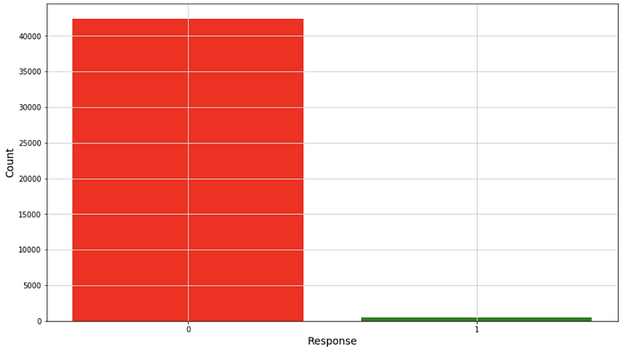
For the second part of the project, the task was to predict whether a person responded to marketing activities. The training set contained 42,962 observations and the same number of features as the demographic data set analyzed during the unsupervised part. However, an additional column called “RESPONSE” served as a label for the supervised training algorithm. It is important to note that the positive class (= person responds to marketing activities) was highly underrepresented within the training data set. Only 532 samples were labeled with 1 (see Figure 10).
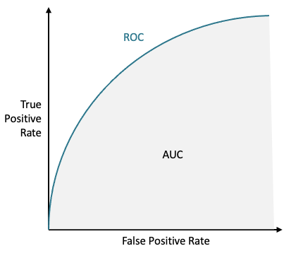
The overall goal was to build a model that performs well on the given task and finally compete in a Kaggle competition against others using a test set that contained 42,833 observations. The score was the ROC AUC. ROC AUC is a is a measurement for the performance of a binary classification model on the positive class. The “True Positive Rate” (TPR) and the “False Positive Rate” (FPR) play an important role here. TPR indicates how many samples of the positive class were correctly classified as positive, whereas FPR indicates how many were incorrectly classified as positive. The ROC curve is plotted with the TPR against the FPR (see Figure 11). AUC stands for “Area Under The (Receiver Operation) Characteristics” and represents the degree of separability.
The ROC AUC is handy for data that is heavily imbalanced. The value can be between 0.0 and 1.0. The higher the value, the better the model is at predicting the positive class. I compared the algorithms by comparing the average validation ROC AUC. This means that it was calculated based on the prediction on data from the hold out validation set.
Initially, I used the same pre-processing steps that I used for the unsupervised part. I tested the following algorithms:
- RandomForestClassifier (0.487 mean validation ROC AUC )
- AdaBoost (0.524 mean validation ROC AUC)
- XGBoost (0.538 mean validation ROC AUC)
For these classifiers, the results were pretty bad. I tried out different parameter configurations and transforming steps, but the performance increased only slightly. Therefore, I suspected that information was lost during my chosen preprocessing approach, so I decided to take a step back and do feature engineering again. Since I assumed that I classified the columns correctly as ordinal, numeric, categorical, and binary, I chose to re-include the columns with type “unknown”. I treated them as ordinal columns and, thus, imputed the median. With these changes, I tested the algorithms again, and the results implied that my assumption was correct:
- RandomForestClassifier (0.585 mean validation ROC AUC)
- AdaBoost (0.719 mean validation ROC AUC)
- XGBoost (0.750 mean validation ROC AUC)
Since I found XGBoost to be the best performing classifier. This result was quite obvious since XGBoost is one of the most powerful machine learning algorithms for tabulated data today. XGBoost is an ensemble algorithm that uses gradient boosted decision trees and is optimized for speed and performance. Compared to other algorithms, XGBoost has some build-in functionalities, such as l1 and l2 regularization. I chose to use it as a foundation for further improvement. I created the following steps to build a pipeline:
steps=[
('scaler', StandardScaler()),
('pca', PCA(explained_variance)),
('smote', SMOTE(sampling_strategy=smote_sampling_strategy, random_state=42)),
('under', RandomUnderSampler(sampling_strategy=under_sampling_strategy, random_state=42)),
('model', model)
]
The transformers scaler and pca were the same as those used during the unsupervised learning part of the project. smote and under were both resampling techniques that can be used to handle imbalanced data. Oversampling increases the number of samples with the minority class while undersampling reduces the number of samples labeled as the majority class. model represents the XGBRegressor. This classifier has the parameter scale_pos_weight, which can also control the balance of positive and negative weights.
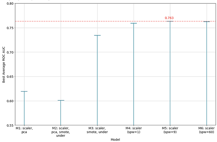
I testet the following combinations of steps:
- M1: Scaling and PCA
- M2: Scaling, PCA, SMOTE and undersampling
- M3: Scaling, SMOTE and undersampling
- M4: Scaling with scale_pos_weight=1 (default)
- M5: Scaling with scale_pos_weight=9
- M6: Scaling with scale_pos_weight=60
I chose to perform RandomizedSearchCV, which is a variant of GridSearch. Here, a combination of parameters is chosen randomly instead of going through every possible configuration. Thus, it is possible to test a broader range of parameters with lesser iterations. I aimed to tune the following parameters since these were found to be the most important for XGBoost.
params = {
'model__learning_rate': [0.01, 0.1, 0.3],
'model__n_estimators': [50, 100, 500],
'model__max_depth': [3, 4, 5],
'model__gamma': [0.5, 1, 1.5, 2, 5],
'model__subsample': [0.6, 0.8, 1.0],
'model__min_child_weight': [1, 5, 10],
}
I chose 20 Iterations per search and performed a 5-fold cross-validation, which resulted in 100 fits for each model configuration. The results can be seen in Figure 12.
The optimal hyperparameter configuration was:
Best parameters:
{'model__subsample': 0.6,
'model__n_estimators': 500,
'model__min_child_weight': 1,
'model__max_depth': 4,
'model__learning_rate': 0.01,
'model__gamma': 5}Best score: 0.7627367405017353
I used the best model to predict the test data set and compete in the Kaggle competition. The model was able to achieve a ROC AUC score of 0.80415. This score is only 0.0065 less than the score of the third place and earned me a place in the top 15 percent of the competition (see Figure 13).

V Summary and further Improvements
In this project, I first analyzed and cleaned up the existing data. Then I scaled the data and applied PCA to reduce the feature dimensionality. Based on 190 principal components, I identified 13 clusters, 3 of which were disproportionately represented in the customer data. All clusters had in common that they contained mostly elderly and affluent individuals.
For the supervised machine learning part, I first used the same transformations as for clustering. However, this did not lead to satisfactory results. My assumption that the dropped features still contained relevant information turned out to be correct, as the new transformation pipeline delivered significantly better results. I tested several algorithms, but XGBoost turned out to be superior. Through hyperparameter tuning, I tested different configurations. The final model was able to achieve a ROC AUC score of 0.80415, which earned me a place in the top 15 percent in the Kaggle competition.
I think there are several approaches to how the ROC AUC score could be further improved. Among others, I believe that further feature engineering could lead to significant improvements. With additional hyperparameter tuning, one could probably achieve some (smaller) improvements. If in the future an algorithm is established that is even better than XGBoost, it would probably be possible to achieve even better scores.
I would like to thank Udacity, Kaggle and Arvato for providing this great data set.
You can find all code in my GitHub.
